Using AMPL Studio
|
Using AMPL Studio |
|
|
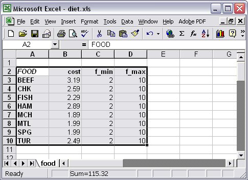
We can use an Excel spreadsheet to store such relational table, by just creating a range that includes the column names; in our example the range is called “Foods” (see Figure 7.1). The name of the range will be used subsequently when reading the data from the spreadsheet into the AMPL Studio model.
Figure 7.1: Excel range as relational table
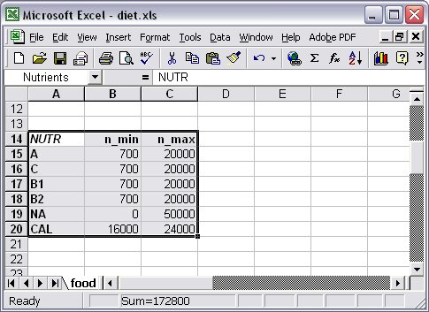
In the same way we can create a second relational table with the set NUTR, which will be the key column, and the two parameters, n_min and n_max, which are indexed over the set NUTR.
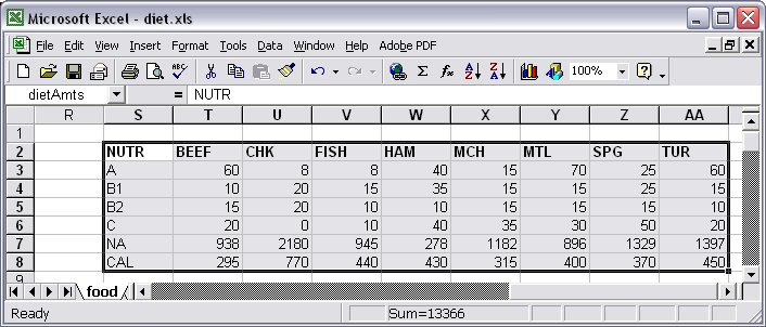
In the Excel spreadsheet we would then create a range, “Nutrients”, that corresponds to this relational table (Figure 7.2).
Figure 72: Excel range “Nutrients” as relational table
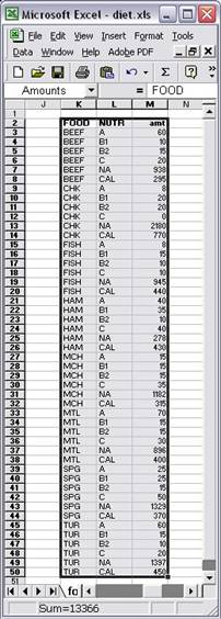
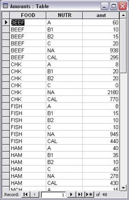
In a similar fashion a third relational table is created for the parameter amt, which is indexed over the two sets NUTR and FOOD. The following table has as key the two columns corresponding to the values for the sets FOOD and NUTR.
The corresponding Excel range, “Amounts”, would look like Figure 7.3.
Figure 7.3: Excel range “Amounts” as relational table
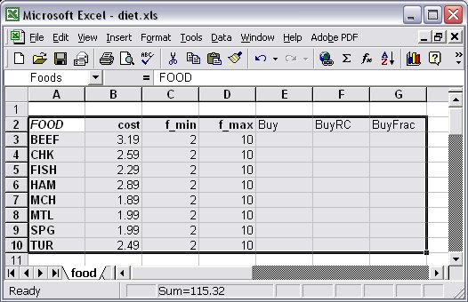
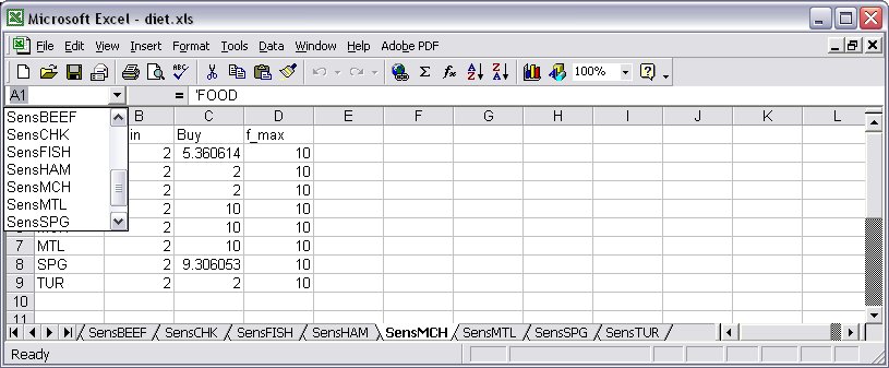
In our Diet.mod model there are other entities indexed over the set FOOD, such as the variables: var Buy {j in FOOD} >= f_min[j], <= f_max[j];Therefore, some assorted result expressions such as Buy, Buy.rc, {j in FOOD} Buy[j]/f_max[j], can be included as output columns in our relational tables. In this case, we can include three new columns to the “Foods” range in our Excel spreadsheet, as in Figure 7.4. The last three columns Buy, BuyRc, and BuyFrac, will be then output columns that will be populated once the model is solved.
Figure 7.4: Excel range “Foods” with input and output columns If we used an Access database to store our relational tables, the relational database for our example might look like Figure 7.5.
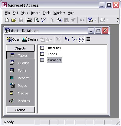
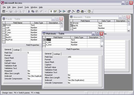
Figure 7.5: Access database for the Diet problem As in the Excel spreadsheet case, we have three relational tables, Foods, Nutrients, and Amounts. The design of the Access relational tables is shown in Figure 7.6.
Figure 7.6: Access Data Tables Design for the Diet problem
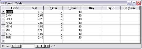
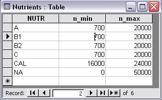
In this case the relational data would be as below.
Figure 7.7: Access Relational Data in Foods table
Figure 7.8: Access Relational Data in Nutrients table
Figure 7.9: Access Relational Data in Amounts table
Now that we have created the relational database, we will see how the relational tables are linked to the AMPL Studio model in order to import and export data from and to the database. Importing data from tablesIn order to use an external relational table, such as the tables created in the section above, for reading only, you should employ a table declaration that specifies a read/write status of IN. The general form of this kind of declaration is table table-name IN string-listopt : key-spec, data-spec, data-spec, … ; Each table declaration has two parts. Before the colon, the declaration provides general information. The table-name is the name by which the table is known within AMPL. The keyword IN states that the default for all non-key table columns will be read-only, i.e., AMPL will use these columns as input columns and will not write out to them. The optional string-list is specific to the database type and access method being used, and we will look into it in more detail in a later section. After the colon, the declaration gives the details of the correspondence between AMPL entities and relational table columns. The key-spec names the key columns, which are surrounded by brackets […]. The data-spec gives the data columns. Data values are subsequently read from the table into AMPL entities by the command read table table-name;
For instance, in our Diet problem example, when we want to read the data from the table “Nutrients”, we would use the following declaration followed by the read command: table dietNutrs IN "ODBC" "TABLES/diet.xls" "Nutrients": NUTR <- [NUTR], n_min, n_max;
read table dietNutrs; In our example the string-list "ODBC" "TABLES/diet.xls" "Nutrients" specifies that we are connecting to the external relational database through an Open Database Connection (ODBC). It also specifies the external file, in this case an Excel spreadsheet “diet.xls” located in the directory “TABLES”. The string “Nutrients” gives the name of the relational table we are declaring. In the second part of the declaration we find the expression NUTR <- [NUTR], which indicates that the entries in the key column NUTR are to be copied into AMPL to define the members of the set NUTR. The expressions n_min and n_max are the names of the other two columns in the relational table from which we will read the values into the parameters n_min and n_max.
In a similar way we can read the data from the “Amounts” relational table
table dietAmts IN "ODBC" "TABLES/diet.xls" "Amounts": [NUTR, FOOD], amt; read table dietAmts;
Reading parameters onlyTo assign values from data columns to like-named AMPL parameters, it suffices to give a bracketed list of key columns and hen a list of data columns. In our Diet problem example, in the simplest case where there is only one key column we could write table Foods IN "ODBC" "TABLES/diet.xls": [FOOD], cost, f_min, f_max; read table Foods;
In the same way, when we want to read multidimensional parameters, the name of each data column must also be the name of an AMPL parameter, and the dimension of the parameter’s indexing set must equal the number of key columns. table Amounts IN "ODBC" "TABLES/diet.xls": [NUTR, FOOD], amt;
read table Amounts;
Values of unindexed (scalar) parameters may be supplied by a relational table that has one row and no key columns, so that each data column contains exactly one value. The corresponding table declaration has an empty key-spec, []. Reading a set and parametersWe can read the members of a set form a table’s key column or columns, at the same time that parameters indexed over that set are read from the data columns. To indicate that a set should be read from a table, the key-spec in the table declaration is written in the form Set-name <- [key-col-spec, key-col-spec,…] The simplest case involves reading a one-dimensional set and the parameters indexed over it. In our Diet problem example we have table Foods IN "ODBC" "TABLES/diet.xls": FOOD <- [FOOD], cost, f_min, f_max;
In this particular case, since the key column [FOOD] is named like the AMPL set FOOD, the table declaration could be abbreviated to table Foods IN "ODBC" "TABLES/diet.xls": [FOOD] IN , cost, f_min, f_max;
For the multidimensional case, an analogous syntax is used fir reading a multidimensional set along with parameters indexed over it. Let’s suppose we had in our Diet.mod the following sets and parameters: set FOOD;set NUTR;set PAIR within {FOOD, NUTR};…param amt {PAIR} >=0;
In this case we would have a table declaration that might look like table Amounts IN "ODBC" "TABLES/diet.xls": PAIR <- [NUTR, FOOD], amt;
Establishing correspondencesSometimes the AMPL model’s set and parameter declarations do not necessarily correspond in all respects to the organization of tables in the external relational databases. One of the most common differences appears in the names amongst the sets and parameters and the corresponding columns in the relational tables. A table declaration can associate a data column with a differently named AMPL parameter by use of a data-spec of the form param-name ~ data-col-name
In our Diet problem example, if we had the following table declaration table Foods IN: [FOOD], cost, f_min ~ lowerlim, f_max ~ upperlim;
We would be saying that the AMPL parameters f_min and f_max would be read from the data columns lowerlim and upperlim in the relational table respectively. In a similar way, when the AMPL index is not named as the corresponding column in the relational table, we would have index ~ key-col-name
This index may then be used in a subscript to the optional param-name in one or more data-specs. Three common cases where we can benefit from this correspondence are as follow. Case 1: as an example, the time periods are counted from 0 in the relational table, but in the model the time periods start counting from 1: table tableName IN: [p ~ PROD, t ~ TIME], market[p,t+1] ~ market, revenue[p,t+1] ~ revenue;
Case 2: the AMPL parameters have subscripts from the same sets but in different orders. In this case key column indexes must be used to provide a correct index order: For example, we have in the AMPL model param market {PROD, 1..T}; param revenue {1..T, PROD}; … we could have a table declaration as follows
table tableName IN: [p ~ PROD, t ~ TIME], market, revenue[t, p] ~ revenue;
Case 3: the values for an AMPL parameter are divided among several database columns. In this case key column indexes can be used to describe the values to be found in each column: For example, if we have the revenue values given in two columns, one for “p1” and in another column for “p2”, the table declaration would be as follows
table tableName IN: [t ~ TIME], revenue[“p1”, t] ~ revenuep1, revenue[“p2”, t] ~ revenuep2;
Reading other valuesAny assignable expression, such as a variable name, a constraint name, a variable or constraint qualified by an assignable suffix, may appear anywhere that a parameter name would be allowed. Therefore, any assignable expression can appear in a table declaration.
In our Diet problem example we could have the following table declaration table Foods IN: FOOD IN, cost, f_min, f_max, Buy, Buy.priority ~ prior;
where we are reading from the table Foods the initial values for the Buy variables, as well as their branching priorities.
Exporting data into tablesIn order to use an external relational table for writing only, you should employ a table declaration that specifies a read/write status of OUT. The general form of this kind of declaration is table table-name OUT string-listopt : key-spec, data-spec, data-spec, … ;
As for the case in which we read data from the table, each table declaration has two parts. Before the colon, the declaration provides general information. The table-name is the name by which the table is known within AMPL. The keyword OUT states that the default for all non-key table columns will be write-only, i.e., AMPL will use these columns as output columns and will not read from them. The optional string-list is specific to the database type and access method being used, and we will look into it in more detail in a later section. After the colon, the declaration gives the details of the correspondence between AMPL entities and relational table columns. The key-spec names the key columns, which are surrounded by brackets […]. The data-spec gives the data columns. Data values are subsequently written to the table by the command write table table-name;
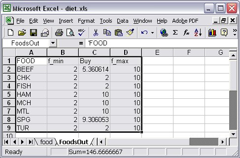
This way the write table command allows writing meaningful results back to the external relational database once the model has been solved. The key-specs and data-specs in the table declaration for writing external tables resemble those for reading. Nevertheless, the range of AMPL expressions allowed when writing is much broader, including essentially all set-valued and numeric-valued expressions. Moreover, whereas the table rows to be read are those of some existing table, the rows to be written must be determined from AMPL expressions in some part of a table declaration. Specifically, rows to be written can be inferred either from the data-specs, or from the key-spec. Each of these alternatives uses a different syntax. Writing rows inferred from the data specificationsIf the key-spec is simply a bracketed list of the names of key columns, [key-col-name, key-col-name,…] then the table declaration works similar to the display command, except that all the items listed in the data-specs must have the same dimension. In the simplest case, the data-specs are the names of model components indexed over the same set. For instance, in our Diet problem example, the table declaration and the write table command table Foods OUT "ODBC" "TABLES/diet.xls" "FoodsOut": [FOOD], f_min, Buy, f_max; … write table Foods; would have as a result a new range named “FoodsOut” as shown in Figure 7.10.
Figure 7.10: Output table range “FoodsOut” in Excel
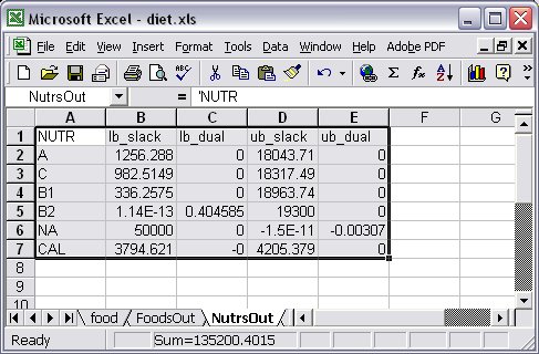
Tables of higher-dimensional sets are handled in the same way, with the number of bracketed key-column names listed in the key-spec being equal to the dimensions of the items in the data-spec. We could also write out to a relational table suffixed variables or constraint names, such as the dual and slack values. In our Diet problem example, we could for instance write out the dual and slack values related to the constraint “diet”: table Nutrients OUT "ODBC" "TABLES/diet.xls" "NutrsOut": [NUTR], diet.lslack ~ lb_slack, diet.ldual ~ lb_dual, diet.uslack ~ ub_slack, diet.udual ~ ub_dual; … write table Nutrients;
which would have as a result a new relational table “NutrsOut” in our Excel Spreadsheet diet.xls, as shown in Figure 7.11.
Figure 7.11: Output table range “NutrsOut” in Excel
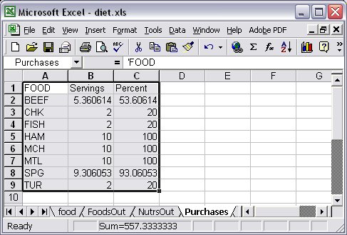
More general expressions for the values in data columns can also be used. Since indexed AMPL expressions are rarely valid column names for a database, they should generally be followed by ~ data-col-name to provide a valid name for the corresponding data table column. For instance, we could have in our Diet problem example the following table declaration: table Purchases OUT "ODBC" "TABLES/diet.xls": [FOOD], Buy ~ Servings, {j in FOOD} 100*Buy[j]/f_max[j] ~ Percent; … write table Purchases;
The resulting relational table is displayed in Figure 7.12.
Figure 7.12: Output table range “Purchases” in Excel
Writing rows inferred from a key specification
We can also use table declarations to write one table row for each member of an explicit specified AMPL set. In this case the key-spec must be of the form set-spec -> [key-col-spec, key-col-spec, …]
This form uses an arrow pointing from left to right, i.e., pointing from an AMPL set to a key column list, indicating that the information will be written from the set into the key columns. The set-spec is composed of an explicit expression, such as the name of an AMPL set, or any other AMPL set-expression enclosed in braces { }. The key-col-spec gives the names of the corresponding key columns in the database.
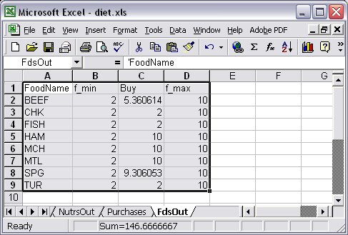
The simplest case of this form would be writing database columns for model components indexed over the same one-dimensional set. In our Diet problem example, we could have table FdsOut OUT "ODBC" "TABLES/diet.xls": FOOD -> [FoodName], f_min, Buy, f_max; … write table FdsOut; giving the relational table shown in Figure 7.13.
Figure 7.13: Output table range “FdsOut” in Excel
or in case we wanted the same name for the table as for the set, we could have written the declaration as table FdsOut OUT "ODBC" "TABLES/diet.xls": [FOOD] OUT, f_min, buy, f_max;
Importing From and Exporting To the Same TableIn the previous sections you have learnt how to import data from an external relational table, and how to export data into a different relational table. There could be cases in which you want to use the same external relational table for both actions, import and export data. In this case you could use two separate table declarations, one to read data, and a second declaration to write data. You may also combine these two declarations into one that specifies some columns to be read and some columns to be written into.
Importing and exporting data using two table declarations
The same external relational table can be read by one table declaration and a read table command, and later on it can be written by another table declaration and a write table command. These two table declarations follow the syntax and rules described in the previous sections.
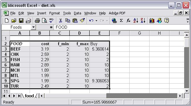
In our Diet problem example, we can have an external relational table “Foods” with some columns that contain input for the model, and other columns that will contain results.
Figure 7.14: Excel range “Foods” with input and output columns
For instance, in Figure 7.14 we have the columns cost, f_min, and f_max as input columns, whereas the columns Buy, BuyRC, and BuyFrac are output columns. This relational table would correspond to the following table declarations: table inputFoods IN "ODBC" "TABLES/diet.xls" "Foods": FOOD <- [FOOD], cost, f_min, f_max;
table outputFoods "ODBC" "TABLES/diet.xls" "Foods": [FOOD], Buy;
Figure 7.15: Input/Output table range “Foods” in ExcelThe user should be careful when using two separate table declarations for input and output from the same table: We could have also used the following table declarations: table inputFoods IN "ODBC" "TABLES/diet.xls" "Foods": FOOD <- [FOOD], cost, f_min, f_max;
table outputFoods OUT "ODBC" "TABLES/diet.xls" "Foods": [FOOD], Buy;
or similarly
table inputFoods IN "ODBC" "TABLES/diet.xls" "Foods": FOOD <- [FOOD], cost, f_min, f_max;
table outputFoods "ODBC" "TABLES/diet.xls" "Foods": [FOOD], Buy OUT;
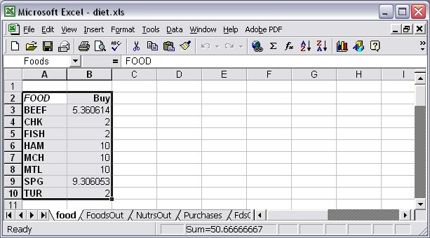
In this case all the data columns in the external relational table “Foods” would have been deleted by the write table outputFoods command, and you would only find the columns specified in the outputFoods table declaration, i.e., the “FOOD” and “Buy” columns:
Figure 7.16: Input/Output table “Foods” if rewriting all columns
Reading and writing using the same table declarationIn many cases a single table declaration suffices to read and write the same external relational table. The key-spec may use the arrow <- to read contents of the key columns into an AMPL set, or use the arrow -> to write members of an AMPL set into the key columns, or even <-> to do both. A data-spec may specify read/write status IN for the columns that will only be read into AMPL, status OUT for the columns that will only be written out from AMPL, or status INOUT for the columns that will be both read and written.
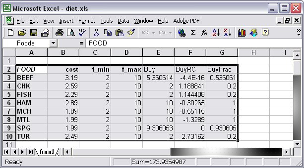
The read table command related to such combined table declaration will read only the keys or data columns that are specified in the table declaration with IN or INOUT read/write status. The write table command related to such combined table declaration will write only the keys or data columns that are specified in the table declaration with OUT or INOUT read/write status. In our Diet problem example, we could use the following table declaration to read and write the Foods table: table dietFoods "ODBC" "TABLES/diet.xls" "Foods": FOOD <- [FOOD], cost IN, f_min IN, f_max IN, Buy OUT, Buy.rc ~ BuyRC OUT, {j in FOOD} Buy[j]/f_max[j] ~ BuyFrac; … read table dietFoods; … write table dietFoods;
and we would obtain the table as in Figure 7.17.
Figure 7.17: Input/Output table “Foods” using one table declaration
Index Collections of Tables and ColumnsSometimes it is convenient to declare an indexed collection of tables, or to define an indexed collection of data columns within a table. This can be done with the table declaration. Indexed collections of tablesThe table declarations can be indexed by following the table-name by an optional {indexing-expr}: table table-name {indexing-expr}opt string-listopt : …
In this case one table is defined for each member of the set specified by the indexing-expr. Individual tables in this collection are denoted by appending a bracketed subscript or subscripts to the table-name. For instance, in our Diet problem example, we could create one different table in our external relational database for each value of the set FOOD: table DietSens {j in FOOD} OUT “ODBC” "TABLES/diet.xls" (“Sens” & j) : [FOOD], f_min, Buy, f_max; …
Which will have as a result the creation of one table per j in FOOD:
Figure 7.18: Tables collection
Indexed collections of data columnsDue to the natural correspondence between data columns of a relational table and indexed collections of entities in an AMPL model, each data-spec in a table declaration normally refers to a different AMPL parameter, variable or expression. However, occasionally the values for one AMPL entity are split among multiple data columns. In this case we can define a collection of data columns, one for each member of a specified indexing set. The general form for specifying an indexed collection of table columns is the following {indexing-expr} < data-spec, data-spec, … >
Each data-spec has any of the forms previously seen. For each member of the set specified by the indexing-expr, AMPL generates one copy of each data-spec within the angle brackets <…>. The indexing-expr also defines one or more dummy indices that run over the index set. These indices are used in expressions within the data-specs, and also appear in string expressions that give the names of columns in the external database. In our Diet problem example, if we have the following table declaration: table dietAmts IN “ODBC” “TABLES/diet.xls”: [i ~ NUTR], {j in FOOD} < amt[i,j] ~ (j) >;
The key-spec [i ~ NUTR] associates the first table column with the set NUTR. The data-spec {j in FOOD} <…> causes AMPL to generate an individual data-spec for each member of the set FOOD. The result would be as displayed in Figure 7.19.
Figure 7.19: Indexed collection of data columns
A similar approach works for writing two-dimensional tables. Standard and Built-in Table HandlersTo work with external database files, AMPL relies on table handlers. These are add-ons, usually in the form of shared or dynamic link libraries that can be loaded as needed. AMPL Studio is distributed with a “standard” table handler that runs under Microsoft Windows and communicates via the Open Database Connectivity (ODBC) application programming interface; it recognizes relational tables in the formats used by Access, Excel, and any other application for which and ODBC driver exists on your computer. As you have seen in the previous examples, AMPL communicates with handlers through the string-list in the table declaration. The form and interpretation of the string-list are specific to each handler. The general form of the string-list in a table declaration for the standard ODBC table handler is “ODBC” “connection-spec” “external-table-spec”opt “verbose”opt
The string “ODBC” indicates that data transfers using this table should employ the standard ODBC handler. The connection-spec identifies the database file name that will be read or written.
The external-table-spec normally gives the name of the relational table, within the specified file that is to be read or written. As we have seen previously, if the table name is omitted, then the name of the relational table is taken to be the same as the table-name of the containing table declaration. The string verbose is used to request diagnostic messages, such as the DSN= string that ODBC reports using.
Using our Diet problem example, three common table-handling statements would be as follows: Case 1: For a Microsoft Access table in a database file diet.mdb located in the TABLES directory: Table Foods IN “ODBC” “TABLES/diet.mdb” : FOOD <- [FOOD], cost, f_min, f_max;
Case 2: For a Microsoft Excel table in a database file diet.xls located in the TABLES directory: Table Foods IN “ODBC” “TABLES/diet.xls” : FOOD <- [FOOD], cost, f_min, f_max;
Case 3: For an ASCII text table in a file Foods.dat located in the TABLES directory:
Table Foods IN “TABLES/Foods.dat”: FOOD <- [FOOD], cost, f_min, f_max;
Solve and Display ResultsAfter solving our Diet problem example we obtain the following solution file.
AmplStudio Modeling System - Copyright (c) 2003-2004, Datumatic Ltd _______________________________________________________________ MODEL.STATISTICS
Problem name :diet Model Filename :Diet.mod Data Filename :Diet2a.dat Date :1:9:2005 Time :20:5 Constraints :6 : Nonzeros S_Constraints :6 Variables :8 : Nonzeros
SOLUTION.RESULT
'Optimal solution found' FortMP 3.2j: LP OPTIMAL SOLUTION, Objective = 118.0594032
DECISION.VARIABLES
Name Activity .uc Reduced Cost _____________________________________________________________ Buy['BEEF'] 5.3606 10.0000 -0.0000 Buy['CHK'] 2.0000 10.0000 1.1888 Buy['FISH'] 2.0000 10.0000 1.1444 Buy['HAM'] 10.0000 10.0000 -0.3027 Buy['MCH'] 10.0000 10.0000 -0.5512 Buy['MTL'] 10.0000 10.0000 -1.3289 Buy['SPG'] 9.3061 10.0000 0.0000 Buy['TUR'] 2.0000 10.0000 2.7316 _____________________________________________________________ CONSTRAINTS Name Slack body dual ____________________________________________________________ diet['A'] 1256.2882 1956.2882 0.0000 diet['B1'] 336.2575 1036.2575 0.0000 diet['B2'] 0.0000 700.0000 0.4046 diet['C'] 982.5149 1682.5149 0.0000 diet['NA'] -0.0000 50000.0000 -0.0031 diet['CAL'] 3794.6206 19794.6206 0.0000 END
We have also seen along the chapter that by using the table declarations and write table commands we can also display the results in an external relational database.
|
|
|
Copyright (c) 2012. Datumatic Ltd. Registration No. 04988675. UK. |